Quantum Error Mitigation (QEM): The Complete Technical Guide
What is Quantum Error Mitigation (QEM)? Quantum Error Mitigation is a suite of software-level classical post-processing protocols designed to reduce computational errors on Noisy Intermediate-Scale Quantum (NISQ) processors. Unlike Quantum Error Correction (QEC), QEM requires zero to minimal physical qubit overhead, directly estimating ideal expectation values ⟨O⟩ from ensembles of noisy measurement data without real-time syndrome feedback.
A superconducting transmon qubit loses coherence in roughly 100 microseconds. A two-qubit gate on today's best hardware carries an error rate between 0.1% and 1%. Sounds small? Run a 200-gate circuit and those errors compound multiplicatively. The output distribution you measure at the end bears only a faint resemblance to the ideal quantum state you intended to prepare. The signal drowns in noise.
This is the NISQ paradox. We have machines with 50, 100, even 1000+ qubits—enough to tackle problems classical supercomputers genuinely struggle with—yet the noise floor is so high that raw results are often scientifically useless. You cannot simply "trust the hardware."
So what do we do? We cannot wait a decade for full fault-tolerant architectures. The answer, and it is the answer the field has converged on with remarkable consensus since 2019, is Quantum Error Mitigation (QEM): a family of techniques that accept noisy hardware as a given and extract accurate physical quantities through clever classical post-processing of measurement data.
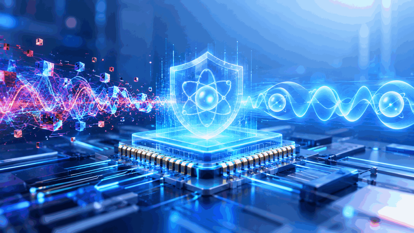
Demystifying Quantum Error Mitigation: Recovering Truth from Noise
Let me be precise about what QEM is, because the term gets mangled constantly in press releases.
Quantum Error Mitigation is not a method that fixes qubits. It does not protect quantum states during computation. It does not add redundancy. Instead, QEM operates on a fundamentally different premise: run your noisy circuit many times, collect a large ensemble of measurement outcomes, and then apply a classical statistical correction to the resulting expectation values to recover what the ideal, noiseless circuit would have produced.
The key insight is this separation of concerns. The quantum hardware does what it does—noisy, imperfect, lossy. The classical processor takes over afterward and performs the intellectual heavy lifting of disentangling signal from noise. QEM is, at its core, a software-and-statistics counterattack against physical hardware imperfection.
This has a profound practical consequence: benchmark QEM protocols (such as ZNE, PEC, and readout mitigation) require zero additional physical qubits—no ancilla arrays, no real-time syndrome measurement, and no active feedback controllers. (While advanced variants like virtual distillation use state copies, mainstream QEM runs on your native chip footprint). You run the same circuit on the same hardware, sample deliberately modified configurations, and allow classical statistical inference to do the rest.
Under the Hood: The Four Main Techniques Driving QEM Today
Zero-Noise Extrapolation (ZNE)
The intuition behind Zero-Noise Extrapolation (ZNE), first proposed by Temme et al., is almost embarrassingly simple.. If noise degrades your result in a predictable way, you can intentionally make the noise worse, observe how the answer degrades, and then extrapolate backward to the zero-noise limit.
Concretely: you run your circuit at the native noise level (scale factor λ = 1). Then you artificially amplify the noise—typically by inserting pairs of identity gates (which are not truly identity on real hardware) or by stretching gate pulse durations—to create effective noise levels at λ = 2, λ = 3, perhaps λ = 4. You measure the observable of interest at each noise level. You now have a set of data points: expectation value versus noise scale factor. Fit a curve (linear, quadratic, Richardson, exponential—choice matters). Extrapolate to λ = 0. That intercept is your mitigated estimate.
Think of it like this: you have a photograph taken through increasingly foggy glass. You cannot remove the fog. But if you photograph the same scene through glass of known, increasing thickness, you can mathematically reconstruct what the image looks like with no glass at all.
ZNE is hardware-agnostic, requires no characterization of the noise model, and has become the default first-line mitigation technique at IBM, Rigetti, and in academic labs worldwide. Its weakness: the extrapolation assumes the noise behaves smoothly and predictably as you scale it. Real hardware sometimes violates this assumption.
Probabilistic Error Cancellation (PEC)
Where ZNE is a blunt extrapolation instrument, Probabilistic Error Cancellation (PEC)—introduced in foundational work on quasi-probability—is a surgical one.. The idea: if you know the exact noise channel acting on your circuit—say, a depolarizing channel with known parameter—you can mathematically invert it. The inverse of a noise channel is generally not a physical quantum operation. It involves quasi-probability distributions with negative weights.
PEC works by decomposing the ideal (noiseless) circuit into a linear combination of implementable noisy circuits, some with negative coefficients. You sample from this decomposition, run each sampled circuit, and combine the results with the appropriate signs. The negative-probability terms effectively subtract the noise contribution.
The analogy that works best: active noise cancellation headphones. The microphone picks up ambient noise, the processor generates an anti-phase signal, and the superposition cancels the unwanted sound. PEC generates "anti-noise" circuits that cancel the physical noise in expectation.
The catch is severe. PEC requires accurate knowledge of the noise model (typically via tomography or cycle benchmarking), and the sampling overhead grows exponentially with circuit depth. For a 50-gate circuit, you might need 10⁴ shots. For a 200-gate circuit, you might need 10⁸ or more. The cost is real.
Readout Error Mitigation
This is the simplest and often the most immediately impactful technique. Quantum measurement is imperfect. A qubit prepared in |0⟩ might be read as "1" with probability 2–5% on current hardware. This is a classical confusion problem.
You characterize the readout error by preparing known states (all-zeros, all-ones, and sometimes superpositions), measuring them, and constructing a confusion matrix M where M[i][j] is the probability of reading outcome i when the true state is j. At runtime, you invert this matrix (or apply a least-squares correction) to your raw measurement histogram. Done.
It is unglamorous. It is also essential. Every serious QEM pipeline starts here.
Clifford Data Regression (CDR) and Symmetry Verification
CDR exploits a clever asymmetry: Clifford circuits can be simulated efficiently on a classical computer (by the Gottesman-Knill theorem), yet they are still quantum circuits that experience the same hardware noise. You generate a training set of near-Clifford circuits, compute their ideal outputs classically, run them on hardware, and learn a linear mapping from noisy to ideal expectation values. You then apply this learned mapping to your target (non-Clifford) circuit.
Symmetry verification takes a different angle. Many physically meaningful quantum states obey conservation laws—particle number conservation, spin symmetry, parity. If your measurement outcome violates these symmetries, it is definitively corrupted by noise. You discard those shots. Simple. Effective. Limited to problems with known symmetries.
The Great Confusion: Quantum Error Mitigation (QEM) vs. Quantum Error Correction (QEC)
Now that the mechanics of QEM are clear, we can address the question that trips up every journalist and every new graduate student entering the field: if QEM is so powerful, why does anyone bother with Quantum Error Correction? Are they not solving the same problem?
No. They are solving fundamentally different problems with fundamentally different philosophies, and conflating them leads to terrible engineering decisions.
QEC is a hardware-level, real-time, state-preserving protocol. It encodes a single logical qubit into many physical qubits (surface code: perhaps 1000+ physical qubits per logical qubit at useful error rates), continuously measures error syndromes, and applies corrections during the computation. The quantum state itself is protected. The computation runs fault-tolerantly.
QEM is a software-level, post-hoc, expectation-value-recovering protocol. The quantum state is not protected. It decoheres. It gets corrupted. QEM accepts this and asks only: "Given that the state was corrupted, can I still extract the correct expectation value of my observable from enough noisy samples?" The answer is yes, at a sampling cost.
Here is the submarine analogy that I find most honest. QEC is like building a submarine with an impossibly expensive, perfectly sealed titanium double hull—no water gets in, ever, and the crew operates in a pristine environment. QEM is like accepting that the hull leaks slightly, installing extremely precise flow sensors, recording exactly how much water enters per second, and then subtracting that water weight from your cargo manifest after the voyage. The submarine still floats. The cargo manifest is still accurate. But the hull is wet.
| Dimension | Quantum Error Mitigation (QEM) | Quantum Error Correction (QEC) |
|---|---|---|
| Core Philosophy | Accept noise; recover expectation values via classical post-processing | Prevent noise from corrupting the quantum state in real time |
| Hardware (Qubit) Overhead | Zero additional qubits required | Massive: 100–1000+ physical qubits per logical qubit |
| Time / Sampling Cost | Exponential growth in required measurement shots with circuit depth | Constant overhead per logical operation (once encoded) |
| Target Era | NISQ | Fault-tolerant era (likely 2030s+) |
| Primary Output | Corrected expectation value ⟨O⟩ of an observable | Protected logical quantum state; arbitrary long computation |
| Real-Time Feedback? | No. Purely post-hoc. | Yes. Continuous syndrome measurement and correction. |
The reason we cannot simply "wait for QEC" is arithmetic. Current hardware has ~1000 physical qubits. A single useful logical qubit under surface code at physical error rates of 10⁻³ requires roughly 1000–2000 physical qubits. A computation needing 100 logical qubits demands 100,000–200,000 physical qubits. We are one to two orders of magnitude away from that. QEM is not a placeholder. It is the only path to scientifically meaningful results on hardware that exists today.
The Engineering Catch: The Hidden Sampling Overhead "Tax"
Here is the engineering trade-off that separates honest QEM research from hype.
QEM trades qubit overhead for sampling overhead. You save physical qubits, but you pay in measurement shots. And this payment is not linear. For PEC, the sampling overhead scales as γ^d, where γ is a factor depending on the noise strength per gate and d is the circuit depth. For typical superconducting hardware with two-qubit gate error rates around 10⁻³, γ ≈ 1.02–1.05. At depth 50, that is a factor of 3–10× more shots. At depth 200, it is 50–1000×. At depth 500, the overhead becomes physically prohibitive—you would need more shots than the age of the universe allows at current repetition rates.
ZNE is more forgiving in practice because it does not require full noise characterization, but its accuracy degrades when the noise model is non-Markovian or when the extrapolation function is poorly chosen. CDR is limited to observables that correlate well with the Clifford training set.
There is no free lunch. QEM extends the useful computational window of NISQ devices from "essentially zero depth" to "perhaps 100–300 gates for specific observables." That is enormously valuable. It is not infinite. Anyone claiming QEM removes the need for better hardware is either confused or selling something.
Real-World Impact: What QEM Unlocks for Scientific Discovery Today
Enough theory. What has QEM actually delivered?
In 2023, IBM's team used ZNE combined with readout mitigation on a 127-qubit Eagle processor to simulate the dynamics of the Ising model at a scale where exact classical tensor-network simulation became intractable. The mitigated quantum results matched known physics in regimes where brute-force classical verification was no longer possible. This was not a toy demonstration. It was a genuine scientific result enabled by mitigation.
In quantum chemistry, variational quantum eigensolver (VQE) calculations of molecular ground-state energies—molecules like H₂O, LiH, and small transition-metal complexes—routinely employ readout mitigation plus ZNE to bring energy estimates within chemical accuracy (1.6 mHartree) of the true ground state. Without mitigation, the same circuits produce energies that are chemically meaningless.
Materials science groups at MIT and ETH Zurich have used symmetry verification combined with CDR to study lattice gauge theories and frustrated spin systems, extracting correlation functions that would be impossible to obtain from raw noisy data.
The pattern is consistent: QEM does not make quantum computers "perfect." It makes them useful for specific, well-defined scientific questions where the observable of interest is a low-weight expectation value and the circuit depth is moderate. That is a narrow but genuinely powerful niche.
Frequently Asked Questions (FAQ)
Can Quantum Error Mitigation solve quantum decoherence?
No. QEM cannot prevent physical decoherence (T1 and T2 relaxation). The qubits still lose phase and population during execution. QEM merely uses classical statistical inference to reconstruct what the expectation value would have been in the absence of that decoherence.
Why can't we use QEM for Shor's Algorithm?
Shor's algorithm requires single-shot state fidelity to read out a specific bitstring factor, whereas QEM reconstructs statistical expectation values (⟨O⟩) across many shots. Furthermore, the sampling overhead of QEM scales exponentially with circuit depth, making it computationally impossible for the millions of gate operations required by Shor's algorithm.
Can QEM be combined with Quantum Error Correction (QEC)?
Yes. Early fault-tolerant systems with imperfect logical gates are expected to use QEM at the logical level. Applying mitigation protocols to slightly noisy logical qubits helps bridge the threshold between early logical demonstrations and true utility-scale fault tolerance.
Contact Us
 (+86) 177 3001 9472
 market@originqc.com