Physical Qubits vs Logical Qubits: From Fragile to Fault-Tolerant
Physical qubits and logical qubits are not competing technologies. One is the raw material; the other is the finished product. Understanding how they differ, and how one becomes the other, is essential to understanding where quantum computing actually stands.
What Is a Physical Qubit?
A physical qubit is a two-level quantum system built from real hardware. The term "qubit" describes the unit of quantum information — the quantum analog of a classical bit — but the physical implementation varies across platforms. The defining feature is not the material but the behavior: a physical qubit can exist in a superposition of its two basis states, typically labeled |0⟩ and |1⟩, and can become entangled with other qubits.
There are several established approaches to building physical qubits:
- Superconducting circuits: Fabricated from Josephson junctions on silicon or sapphire wafers. These operate at microwave frequencies and require cryogenic temperatures below 20 millikelvin. Gate times are on the order of 10-100 nanoseconds. Coherence times typically range from 50 to 300 microseconds.
- Trapped ions: Individual atomic ions — commonly ytterbium, calcium, or barium — suspended in vacuum by electromagnetic fields. Quantum states are encoded in hyperfine or optical transitions. Gate operations use laser pulses. Coherence times can exceed several seconds because the ions are well isolated from the environment.
- Neutral atoms: Atoms such as rubidium or cesium held in optical tweezers — tightly focused laser beams that trap individual atoms at precise positions. Rydberg states provide the interaction mechanism for two-qubit gates. Coherence times range from milliseconds to seconds.
- Photonic qubits: Quantum information encoded in properties of individual photons, such as polarization, time-bin, or path. These operate at room temperature and are naturally suited for quantum communication, but two-qubit gates are more challenging to implement deterministically.
Every physical qubit platform shares one characteristic: imperfection. Each gate operation introduces a small probability of error. Typical two-qubit gate error rates range from 0.1% to 1% across leading platforms. The qubit also loses its quantum state through decoherence — the process by which interaction with the environment destroys superposition. The combination of gate errors and decoherence limits the depth of quantum circuits you can run before the output becomes noise.
What Is a Logical Qubit?
A logical qubit is quantum information encoded across multiple physical qubits in a way that protects it from errors. The logical qubit is not a physical object. You cannot isolate it on a chip or point to a single component and say "that is the logical qubit." It is a distributed quantum state — a pattern of entanglement spread across many physical components.
The construction works through quantum error correction. Information stored in a single physical qubit is distributed across an array of physical qubits using a specific code. The code creates redundancy: the same logical information exists in the collective state of the group, not in any individual member. When errors occur on individual physical qubits, the code detects them through syndrome measurements and applies corrections before the errors propagate.
The key principle is that measuring the logical qubit directly would collapse its quantum state. So error correction uses ancilla qubits — auxiliary physical qubits — to perform indirect measurements that reveal whether an error occurred without revealing what the stored quantum information is. These syndrome measurements identify the error type and location. A decoder then determines the most likely correction to apply.
The most widely studied error correction code is the surface code. It arranges physical qubits in a two-dimensional lattice where each qubit interacts only with its nearest neighbors. This locality constraint makes the surface code practical for real hardware, where long-range connectivity is expensive or impossible. The surface code has a relatively high error threshold of approximately 1%, meaning physical qubits need to be better than 99% accurate for the code to work at all.
The Core Difference
The distinction between physical and logical qubits comes down to three dimensions: stability, structure, and purpose.
A physical qubit is a hardware component subject to the laws of physics without any protection layer. It decoheres on its own timescale. Every gate you apply degrades its state slightly. Run enough operations and the information is gone. A logical qubit, by contrast, is actively maintained. Error correction constantly monitors for corruption and repairs it. The logical qubit's lifetime is not determined by the physics of a single component but by the mathematics of the code and the number of physical qubits you invest.
Structurally, a physical qubit is a single entity — one circuit, one atom, one photon. A logical qubit is a collective state. The relationship is similar to how a RAID array of hard drives presents itself as a single logical drive to the operating system. The difference is that quantum error correction must preserve not just data but the phase relationships that make quantum computation possible.
In terms of purpose, physical qubits are what you build. Logical qubits are what you compute with. A quantum algorithm is written in terms of logical operations on logical qubits. The translation from logical to physical — the compilation of logical gates into sequences of physical gates, along with the continuous error correction cycle — is handled by the control system.
How Physical Qubits Become Logical Qubits
The encoding process begins by preparing a group of physical qubits in a specific entangled state defined by the error correction code. For the surface code, this means initializing data qubits and ancilla qubits, then performing a series of stabilizer measurements. Each stabilizer is a multi-qubit operator — typically a product of Pauli X or Pauli Z operators on four neighboring qubits — whose eigenvalue tells you whether the local state is consistent with the code space.
The ancilla qubits measure these stabilizers repeatedly. If all stabilizers return +1, the system is in the code space and no errors are detected. If a stabilizer returns -1, it signals an error on one of the qubits involved. By tracking which stabilizers flip over time, the decoder reconstructs the most likely error chain and applies a correction.
The code distance, denoted as d, is the central parameter. It represents the minimum number of physical errors required to create an uncorrectable logical error. For the surface code, a distance-d code requires approximately d-squared physical qubits to encode one logical qubit. The logical error rate scales roughly as (p/p_th) raised to the power of (d+1)/2, where p is the physical error rate and p_th is the threshold — about 1% for the surface code.
Here is what that means in practice. If your physical qubits have a 0.1% error rate and you use a surface code with distance d = 15, the logical error rate drops to approximately 10 to the power of -15 — effectively zero for most computations. But d = 15 requires roughly 225 physical qubits for a single logical qubit. At current error rates of 0.5-1%, you would need distances of 25 or higher, pushing the physical qubit count per logical qubit into the thousands.
Physical vs Logical Qubits: Key Comparisons
| Property | Physical Qubit | Logical Qubit |
|---|---|---|
| Definition | A single two-level quantum system implemented in hardware | Quantum information encoded across multiple physical qubits via error correction |
| Physical existence | A tangible component — a circuit, an atom, or a photon | A distributed quantum state with no single physical location |
| Coherence time | Microseconds to seconds, depending on platform | Effectively unlimited as long as error correction operates below threshold |
| Error rate per operation | 0.1% to 1% for two-qubit gates on leading platforms | Can be suppressed to 10^-15 or lower with sufficient code distance |
| Resource requirement | One hardware unit | Hundreds to thousands of physical qubits plus continuous error correction overhead |
| Current status | Commercially available with processors of 50-1,000+ qubits | Experimental demonstrations with 1-2 logical qubits; not yet at application scale |
| Computation model | Used in NISQ-era devices for shallow circuits | Required for fault-tolerant quantum computing and deep algorithms |
| Measurement | Direct measurement collapses the quantum state | Indirect syndrome measurements detect errors without collapsing logical information |
Why the Physical-to-Logical Ratio Matters
The number of physical qubits needed per logical qubit is the bottleneck that defines the timeline for practical quantum computing. Consider Shor's algorithm for factoring a 2,048-bit number — the computation relevant to breaking RSA-2048 encryption. Estimates suggest this requires roughly 20 million physical qubits under current error rates. That number breaks down as approximately 4,000 logical qubits, each encoded using about 5,000 physical qubits, plus additional overhead for state distillation and gate teleportation.
The ratio is not fixed. It depends on three variables: the physical error rate, the error correction code, and the target logical error rate for your application. Improving physical qubit quality from 1% error rate to 0.1% reduces the required code distance dramatically. A physical error rate of 0.01% — two orders of magnitude better — could push the ratio down to a few hundred physical qubits per logical qubit.
This is why the industry is shifting its focus. For years, press releases competed on physical qubit counts. A 100-qubit processor was newsworthy; a 1,000-qubit processor was a milestone. But physical qubit count without error correction is like counting transistors on a chip where half of them produce wrong answers. The meaningful metric is logical qubit count, weighted by the code distance and the resulting logical error rate. The field has begun measuring progress this way, and it changes the competitive landscape entirely.
The path forward involves improving physical qubit quality while simultaneously developing more efficient error correction codes. Alternatives to the surface code — such as low-density parity-check codes, color codes, and bosonic codes — promise lower overhead for the same logical error rate. Some approaches reduce the physical-to-logical ratio by an order of magnitude in theory, but they require hardware capabilities that are not yet mature, such as high-fidelity multi-qubit gates or long-range connectivity.
FAQ
How many physical qubits make one logical qubit?
The number depends on the error rate of the physical qubits and the error correction code used. With current superconducting qubit error rates around 0.1-1%, estimates range from 1,000 to 10,000 physical qubits per logical qubit using surface codes. As hardware improves and error rates drop toward 0.01%, that ratio could fall to a few hundred. The exact number is determined by the code distance needed to suppress errors below your application's threshold.
Do logical qubits exist today or are they still theoretical?
Logical qubits have been demonstrated experimentally. In 2023, researchers created a logical qubit using neutral atoms that outperformed its individual physical components, marking a milestone called "breakeven." Multiple teams have since shown logical qubits with superconducting circuits, trapped ions, and photonic systems. These demonstrations are small-scale proof-of-concept experiments, not production-ready hardware. The challenge now is scaling from one or two logical qubits to the hundreds or thousands needed for real applications.
Which is more important for quantum computing: more physical qubits or better logical qubits?
Raw physical qubit count matters only up to a point. A machine with 1,000 noisy physical qubits cannot factor a 2,048-bit number. A machine with 50 logical qubits might. The field is shifting from competing on physical qubit counts to competing on logical qubit quality, which means lower error rates and higher code distances. The metric that actually determines computational power is the number of reliable logical operations you can perform before the system fails, not how many physical qubits sit on the chip.
Why do logical qubits require so many physical qubits?
Quantum error correction works by spreading one piece of quantum information across many physical qubits in an entangled state. The redundancy allows the system to detect and correct errors without directly measuring the data, which would collapse it. Surface codes, the leading approach, arrange physical qubits in a two-dimensional grid where each data qubit is surrounded by ancilla qubits that perform syndrome measurements. A code distance of d requires roughly d-squared physical qubits, and you need a large d to suppress errors enough for deep circuits.
Contact Us
 (+86) 177 3001 9472
 market@originqc.com